通信原理基于matlab的计算机仿真

《通信原理基于matlab的计算机仿真》由会员分享，可在线阅读，更多相关《通信原理基于matlab的计算机仿真（30页珍藏版）》请在装配图网上搜索。

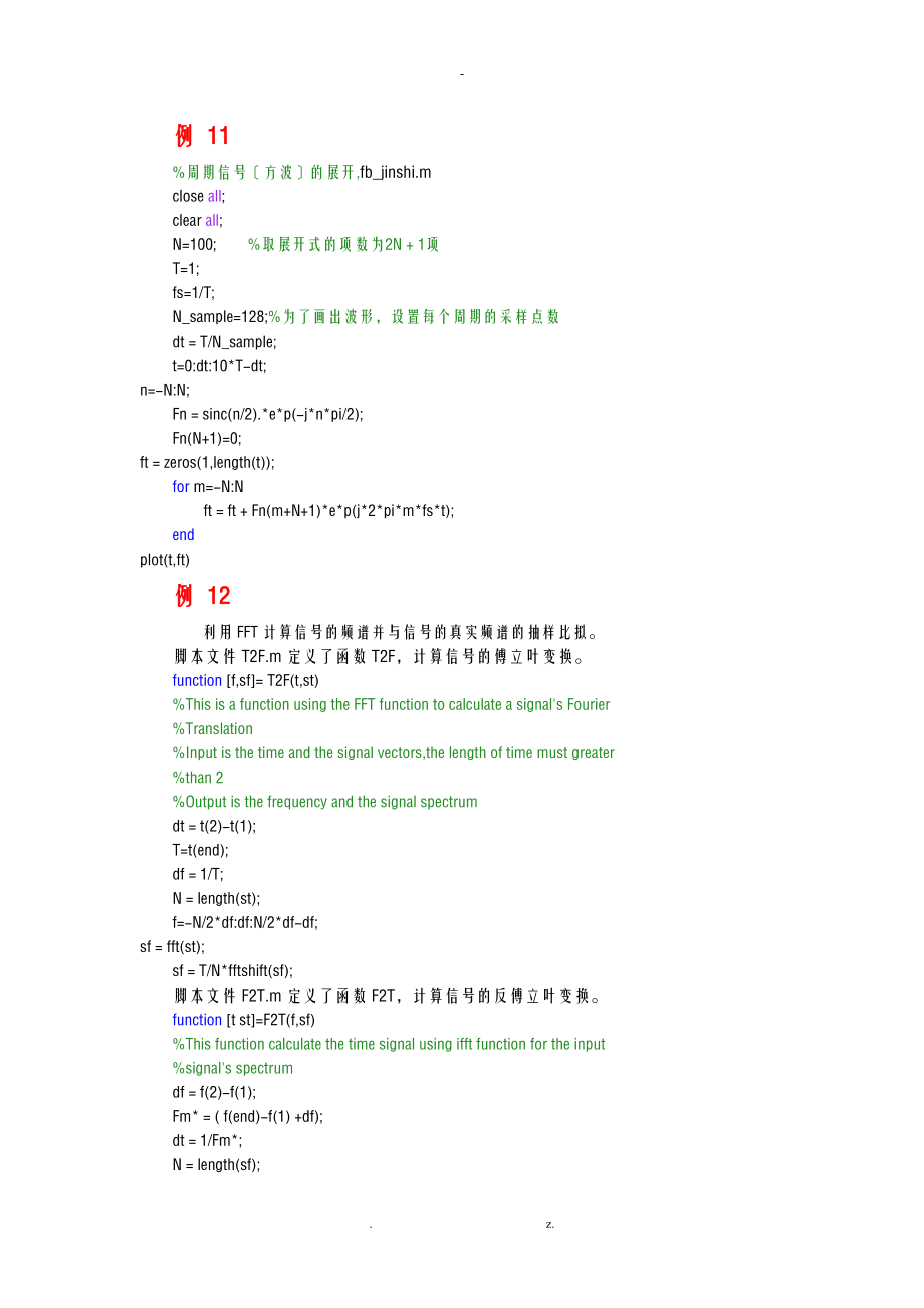
1、-例 11%周期信号方波的展开,fb_jinshi.mclose all;clear all;N=100; %取展开式的项数为2N1项T=1;fs=1/T;N_sample=128;%为了画出波形，设置每个周期的采样点数dt = T/N_sample;t=0:dt:10*T-dt;n=-N:N;Fn = sinc(n/2).*e*p(-j*n*pi/2);Fn(N+1)=0;ft = zeros(1,length(t);for m=-N:N ft = ft + Fn(m+N+1)*e*p(j*2*pi*m*fs*t);endplot(t,ft)例 12利用FFT计算信号的频谱并与信号的真实频谱

2、的抽样比拟。脚本文件T2F.m定义了函数T2F，计算信号的傅立叶变换。function f,sf= T2F(t,st)%This is a function using the FFT function to calculate a signals Fourier%Translation%Input is the time and the signal vectors,the length of time must greater%than 2%Output is the frequency and the signal spectrumdt = t(2)-t(1);T=t(end);df =

3、 1/T;N = length(st);f=-N/2*df:df:N/2*df-df;sf = fft(st);sf = T/N*fftshift(sf);脚本文件F2T.m定义了函数F2T，计算信号的反傅立叶变换。function t st=F2T(f,sf)%This function calculate the time signal using ifft function for the input%signals spectrumdf = f(2)-f(1);Fm* = ( f(end)-f(1) +df);dt = 1/Fm*;N = length(sf);T = dt*N;%t=

4、-T/2:dt:T/2-dt;t = 0:dt:T-dt;sff = fftshift(sf);st = Fm*ifft(sff);另写脚本文件fb_spec.m如下：%方波的傅氏变换, fb_spec.mclear all;close all;T=1;N_sample = 128;dt=T/N_sample;t=0:dt:T-dt;st=ones(1,N_sample/2), -ones(1,N_sample/2); %方波一个周期subplot(211);plot(t,st);a*is(0 1 -2 2);*label(t);ylabel(s(t);subplot(212);f sf=T2

5、F(t,st); %方波频谱plot(f,abs(sf); hold on;a*is(-10 10 0 1);*label(f);ylabel(|S(f)|);%根据傅氏变换计算得到的信号频谱相应位置的抽样值sff= T2*j*pi*f*0.5.*e*p(-j*2*pi*f*T).*sinc(f*T*0.5).*sinc(f*T*0.5);plot(f,abs(sff),r-)例13%信号的能量计算或功率计算,sig_pow.mclear all;close all;dt = 0.01;t = 0:dt:5;s1 = e*p(-5*t).*cos(20*pi*t);s2 = cos(20*pi

6、*t);E1 = sum(s1.*s1)*dt; %s1(t)的信号能量P2 = sum(s2.*s2)*dt/(length(t)*dt); %s2(t)的信号功率sf1 s1f= T2F(t,s1);f2 s2f= T2F(t,s2);df = f1(2)-f1(1);E1_f = sum(abs(s1f).2)*df; %s1(t)的能量,用频域方式计算df = f2(2)-f2(1);T = t(end);P2_f = sum(abs(s2f).2)*df/T; %s2(t)的功率，用频域方式计算figure(1)subplot(211)plot(t,s1);*label(t); yl

7、abel(s1(t); subplot(212)plot(t,s2)*label(t); ylabel(s2(t); 例14%方波的傅氏变换，sig_band.mclear all;close all;T=1;N_sample = 128;dt=1/N_sample;t=0:dt:T-dt;st=ones(1,N_sample/2) -ones(1,N_sample/2);df=0.1/T;F* = 1/dt;f=-F*:df:F*-df;%根据傅氏变换计算得到的信号频谱sff= T2*j*pi*f*0.5.*e*p(-j*2*pi*f*T).*sinc(f*T*0.5).*sinc(f*T*

8、0.5);plot(f,abs(sff),r-)a*is(-10 10 0 1);hold on;sf_ma* = ma*(abs(sff);line(f(1) f(end),sf_ma* sf_ma*);line(f(1) f(end),sf_ma*/sqrt(2) sf_ma*/sqrt(2); %交点处为信号功率下降3dB处Bw_eq = sum(abs(sff).2)*df/T/sf_ma*.2; %信号的等效带宽例 15%带通信号经过带通系统的等效基带表示，sig_bandpass.mclear all;close all;dt = 0.01;t = 0:dt:5;s1 = e*p(

9、-t).*cos(20*pi*t); %输入信号f1 s1f= T2F(t,s1); %输入信号的频谱s1_lowpass = hilbert(s1).*e*p(-j*2*pi*10*t); %输入信号的等效基带信号f2 s2f=T2F(t,s1_lowpass); %输入等效基带信号的频谱h2f = zeros(1,length(s2f);a b=find( abs(s1f)=ma*(abs(s1f) ); %找到带通信号的中心频率h2f( 201-25:201+25 )= 1;h2f( 301-25:301+25) = 1;h2f = h2f.*e*p(-j*2*pi*f2); %参加线性

10、相位，t1 h1 = F2T(f2,h2f); %带通系统的冲激响应h1_lowpass = hilbert(h1).*e*p(-j*2*pi*10*t1); %等效基带系统的冲激响应figure(1)subplot(521);plot(t,s1);*label(t); ylabel(s1(t); title(带通信号);subplot(523);plot(f1,abs(s1f);*label(f); ylabel(|S1(f)|); title(带通信号幅度谱);subplot(522)plot(t,real(s1_lowpass);*label(t);ylabel(Res_l(t);tit

11、le(等效基带信号的实部);subplot(524)plot(f2,abs(s2f);*label(f);ylabel(|S_l(f)|);title(等效基带信号的幅度谱);%画带通系统及其等效基带的图subplot(525)plot(f2,abs(h2f);*label(f);ylabel(|H(f)|);title(带通系统的传输响应幅度谱);subplot(527)plot(t1,h1);*label(t);ylabel(h(t);title(带通系统的冲激响应);subplot(526)f3 hlf=T2F(t1,h1_lowpass);plot(f3,abs(hlf);*label

12、(f);ylabel(|H_l(f)|);title(带通系统的等效基带幅度谱);subplot(528)plot(t1,h1_lowpass);*label(t);ylabel(h_l(t);title(带通系统的等效基带冲激响应);%画出带通信号经过带通系统的响应 及 等效基带信号经过等效基带系统的响应tt = 0:dt:t1(end)+t(end);yt = conv(s1,h1);subplot(529)plot(tt,yt);*label(t);ylabel(y(t);title(带通信号与带通系统响应的卷积)ytl = conv(s1_lowpass,h1_lowpass).*e*

13、p(j*2*pi*10*tt);subplot(5,2,10)plot(tt,real(yt);*label(t);ylabel(y_l(t)cos(20*pi*t);title(等效基带与等效基带系统响应的卷积中心频率载波)例 1-6%例：窄带高斯过程，文件 zdpw.mclear all; close all;N0=1; %双边功率谱密度fc=10; %中心频率B=1; %带宽dt=0.01;T=100;t=0:dt:T-dt;%产生功率为N0*B的高斯白噪声P = N0*B;st = sqrt(P)*randn(1,length(t);%将上述白噪声经过窄带带通系统，f,sf = T2F

14、(t,st); %高斯信号频谱figure(1)plot(f,abs(sf); %高斯信号的幅频特性tt gt=bpf(f,sf,fc-B/2,fc+B/2); %高斯信号经过带通系统glt = hilbert(real(gt); %窄带信号的解析信号，调用hilbert函数得到解析信号glt = glt.*e*p(-j*2*pi*fc*tt);ff,glf=T2F( tt, glt );figure(2)plot(ff,abs(glf);*label(频率(Hz); ylabel(窄带高斯过程样本的幅频特性)figure(3)subplot(411);plot(tt,real(gt);tit

15、le(窄带高斯过程样本)subplot(412)plot(tt,real(glt).*cos(2*pi*fc*tt)-imag(glt).*sin(2*pi*fc*tt)title(由等效基带重构的窄带高斯过程样本)subplot(413)plot(tt,real(glt);title(窄带高斯过程样本的同相分量)subplot(414)plot(tt,imag(glt);*label(时间t(秒); title(窄带高斯过程样本的正交分量)%求窄带高斯信号功率;注：由于样本的功率近似等于随机过程的功率，因此可能出现一些偏差P_gt=sum(real(gt).2)/T;P_glt_real =

16、 sum(real(glt).2)/T;P_glt_imag = sum(imag(glt).2)/T;%验证窄带高斯过程的同相分量、正交分量的正交性a = real(glt)*(imag(glt)/T;用到的子函数function t,st=bpf(f,sf,B1,B2)%This function filter an input at frequency domain by an ideal bandpass filter%Inputs:% f: frequency samples% sf: input data spectrum samples% B1: bandpasss lower

17、frequency% B2: bandpasss higher frequency %Outputs:% t: frequency samples% st: output datas time samplesdf = f(2)-f(1);T = 1/df;hf = zeros(1,length(f);bf = floor( B1/df ): floor( B2/df ) ;bf1 = floor( length(f)/2 ) + bf;bf2 = floor( length(f)/2 ) - bf;hf(bf1)=1/sqrt(2*(B2-B1);hf(bf2)=1/sqrt(2*(B2-B1

18、);yf=hf.*sf.*e*p(-j*2*pi*f*0.1*T);t,st=F2T(f,yf);例 1-7%显示模拟调制的波形及解调方法DSB，文件mdsb.m%信源close all;clear all;dt = 0.001; %时间采样间隔 fm=1; %信源最高频率fc=10; %载波中心频率T=5; %信号时长t = 0:dt:T; mt = sqrt(2)*cos(2*pi*fm*t); %信源%N0 = 0.01; %白噪单边功率谱密度%DSB modulations_dsb = mt.*cos(2*pi*fc*t);B=2*fm;%noise = noise_nb(fc,B,N

19、0,t);%s_dsb=s_dsb+noise;figure(1)subplot(311)plot(t,s_dsb);hold on; %画出DSB信号波形plot(t,mt,r-); %标示mt的波形title(DSB调制信号);*label(t);%DSB demodulationrt = s_dsb.*cos(2*pi*fc*t);rt = rt-mean(rt);f,rf = T2F(t,rt);t,rt = lpf(f,rf,2*fm);subplot(312)plot(t,rt); hold on;plot(t,mt/2,r-);title(相干解调后的信号波形与输入信号的比拟);

20、*label(t)subplot(313)f,sf=T2F(t,s_dsb);psf = (abs(sf).2)/T;plot(f,psf);a*is(-2*fc 2*fc 0 ma*(psf);title(DSB信号功率谱);*label(f);function t st=lpf(f,sf,B)%This function filter an input data using a lowpass filter%Inputs:f: frequency samples% sf: input data spectrum samples% B: lowpasss bandwidth with a r

21、ectangle lowpass%Outputs: t: time samples% st: output datas time samplesdf = f(2)-f(1);T = 1/df;hf = zeros(1,length(f);bf = -floor( B/df ): floor( B/df ) + floor( length(f)/2 );hf(bf)=1;yf=hf.*sf;t,st=F2T(f,yf);st = real(st);例1-8%显示模拟调制的波形及解调方法AM,文件mam.m%信源close all;clear all;dt = 0.001; %时间采样间隔 fm=

22、1; %信源最高频率fc=10; %载波中心频率T=5; %信号时长t = 0:dt:T; mt = sqrt(2)*cos(2*pi*fm*t); %信源%N0 = 0.01; %白噪单边功率谱密度%AM modulationA=2;s_am = (A+mt).*cos(2*pi*fc*t);B = 2*fm; %带通滤波器带宽%noise = noise_nb(fc,B,N0,t); %窄带高斯噪声产生%s_am = s_am + noise;figure(1)subplot(311)plot(t,s_am);hold on; %画出AM信号波形plot(t,A+mt,r-); %标示AM

23、的包络title(AM调制信号及其包络);*label(t);%AM demodulationrt = s_am.*cos(2*pi*fc*t); %相干解调rt = rt-mean(rt);f,rf = T2F(t,rt);t,rt = lpf(f,rf,2*fm); %低通滤波subplot(312)plot(t,rt); hold on;plot(t,mt/2,r-);title(相干解调后的信号波形与输入信号的比拟);*label(t)subplot(313)f,sf=T2F(t,s_am);psf = (abs(sf).2)/T;plot(f,psf);a*is(-2*fc 2*fc

24、 0 ma*(psf);title(AM信号功率谱);*label(f);例 1-9%显示模拟调制的波形及解调方法SSB，文件mssb.m%信源close all;clear all;dt = 0.001; %时间采样间隔 fm=1; %信源最高频率fc=10; %载波中心频率T=5; %信号时长t = 0:dt:T; mt = sqrt(2)*cos(2*pi*fm*t); %信源%N0 = 0.01; %白噪单边功率谱密度%SSB modulations_ssb = real( hilbert(mt).*e*p(j*2*pi*fc*t) );B=fm;%noise = noise_nb(f

25、c,B,N0,t);%s_ssb=s_ssb+noise;figure(1)subplot(311)plot(t,s_ssb);hold on; %画出SSB信号波形plot(t,mt,r-); %标示mt的波形title(SSB调制信号);*label(t);%SSB demodulationrt = s_ssb.*cos(2*pi*fc*t);rt = rt-mean(rt);f,rf = T2F(t,rt);t,rt = lpf(f,rf,2*fm);subplot(312)plot(t,rt); hold on;plot(t,mt/2,r-);title(相干解调后的信号波形与输入信号

26、的比拟);*label(t)subplot(313)f,sf=T2F(t,s_ssb);psf = (abs(sf).2)/T;plot(f,psf);a*is(-2*fc 2*fc 0 ma*(psf);title(SSB信号功率谱);*label(f);例 2-0%显示模拟调制的波形及解调方法VSB，文件mvsb.m%信源close all;clear all;dt = 0.001; %时间采样间隔 fm=5; %信源最高频率fc=20; %载波中心频率T=5; %信号时长t = 0:dt:T; mt = sqrt(2)*( cos(2*pi*fm*t)+sin(2*pi*0.5*fm*t

27、) ); %信源%VSB modulations_vsb = mt.*cos(2*pi*fc*t);B=1.2*fm;f,sf = T2F(t,s_vsb);t,s_vsb = vsbpf(f,sf,0.2*fm,1.2*fm,fc);figure(1)subplot(311)plot(t,s_vsb);hold on; %画出VSB信号波形plot(t,mt,r-); %标示mt的波形title(VSB调制信号);*label(t);%VSB demodulationrt = s_vsb.*cos(2*pi*fc*t); f,rf = T2F(t,rt);t,rt = lpf(f,rf,2*

28、fm);subplot(312)plot(t,rt); hold on;plot(t,mt/2,r-);title(相干解调后的信号波形与输入信号的比拟);*label(t)subplot(313)f,sf=T2F(t,s_vsb);psf = (abs(sf).2)/T;plot(f,psf);a*is(-2*fc 2*fc 0 ma*(psf);title(VSB信号功率谱);*label(f);function t,st=vsbpf(f,sf,B1,B2,fc)%This function filter an input by an residual bandpass filter%In

29、puts: f: frequency samples% sf: input data spectrum samples% B1: residual bandwidth% B2: highest freq of the basedband signal %Outputs: t: frequency samples% st: output datas time samplesdf = f(2)-f(1);T = 1/df;hf = zeros(1,length(f);bf1 = floor( (fc-B1)/df ): floor( (fc+B1)/df ) ;bf2 = floor( (fc+B

30、1)/df )+1: floor( (fc+B2)/df );f1 = bf1 + floor( length(f)/2 ) ;f2 = bf2 + floor( length(f)/2 ) ;stepf = 1/length(f1);hf(f1)=0:stepf:1-stepf;hf(f2)=1;f3 = -bf1 + floor( length(f)/2 ) ;f4 = -bf2 + floor( length(f)/2) ;hf(f3)=0:stepf:(1-stepf);hf(f4)=1;yf=hf.*sf;t,st=F2T(f,yf);st = real(st);例 2-1%显示模拟

31、调制的波形及解调方法AM、DSB、SSB, %信源close all;clear all;dt = 0.001;fm=1;fc=10;t = 0:dt:5;mt = sqrt(2)*cos(2*pi*fm*t);N0 = 0.1;%AM modulationA=2;s_am = (A+mt).*cos(2*pi*fc*t);B = 2*fm;noise = noise_nb(fc,B,N0,t);s_am = s_am + noise;figure(1)subplot(321)plot(t,s_am);hold on;plot(t,A+mt,r-);%AM demodulationrt = s

32、_am.*cos(2*pi*fc*t);rt = rt-mean(rt);f,rf = T2F(t,rt);t,rt = lpf(f,rf,2*fm);title(AM信号);*label(t);subplot(322)plot(t,rt); hold on;plot(t,mt/2,r-);title(AM解调信号);*label(t);%DSB modulations_dsb = mt.*cos(2*pi*fc*t);B=2*fm;noise = noise_nb(fc,B,N0,t);s_dsb=s_dsb+noise;subplot(323)plot(t,s_dsb);hold on;p

33、lot(t,mt,r-);title(DSB信号);*label(t);%DSB demodulationrt = s_dsb.*cos(2*pi*fc*t);rt = rt-mean(rt);f,rf = T2F(t,rt);t,rt = lpf(f,rf,2*fm);subplot(324)plot(t,rt); hold on;plot(t,mt/2,r-);title(DSB解调信号);*label(t);%SSB modulations_ssb = real( hilbert(mt).*e*p(j*2*pi*fc*t) );B=fm;noise = noise_nb(fc,B,N0,

34、t);s_ssb=s_ssb+noise;subplot(325)plot(t,s_ssb);title(SSB信号);*label(t);%SSB demodulationrt = s_ssb.*cos(2*pi*fc*t);rt = rt-mean(rt);f,rf = T2F(t,rt);t,rt = lpf(f,rf,2*fm);subplot(326)plot(t,rt); hold on;plot(t,mt/2,r-);title(SSB解调信号);*label(t);function out = noise_nb(fc,B,N0,t)%output the narrow band

35、 gaussian noise sample with single-sided power spectrum N0%at carrier frequency equals fc and bandwidth euqals Bdt = t(2)-t(1);Fm* = 1/dt;n_len = length(t);p = N0*Fm*;rn = sqrt(p)*randn(1,n_len);f,rf = T2F(t,rn);t,out = bpf(f,rf,fc-B/2,fc+B/2);例 2-2%FM modulation and demodulation，mfm.mclear all;clos

36、e all;Kf = 5;fc = 10;T=5;dt=0.001;t = 0:dt:T;%信源fm= 1;%mt = cos(2*pi*fm*t) + 1.5*sin(2*pi*0.3*fm*t); %信源信号mt = cos(2*pi*fm*t); %信源信号%FM 调制A = sqrt(2);%mti = 1/2/pi/fm*sin(2*pi*fm*t) -3/4/pi/0.3/fm*cos(2*pi*0.3*fm*t); %mt的积分函数mti = 1/2/pi/fm*sin(2*pi*fm*t) ; %mt的积分函数st = A*cos(2*pi*fc*t + 2*pi*Kf*mti

37、);figure(1)subplot(311);plot(t,st); hold on;plot(t,mt,r-);*label(t);ylabel(调频信号)subplot(312)f sf = T2F(t,st);plot(f, abs(sf);a*is(-25 25 0 3)*label(f);ylabel(调频信号幅度谱)%FM 解调for k=1:length(st)-1 rt(k) = (st(k+1)-st(k)/dt;endrt(length(st)=0;subplot(313)plot(t,rt); hold on;plot(t,A*2*pi*Kf*mt+A*2*pi*fc,

38、r-);*label(t);ylabel(调频信号微分后包络)例 2-3%数字基带信号的功率谱密度 digit_baseband.mclear all;close all;Ts=1;N_sample = 8; %每个码元的抽样点数dt = Ts/N_sample; %抽样时间间隔N = 1000; %码元数t = 0:dt:(N*N_sample-1)*dt;gt1 = ones(1,N_sample); %NRZ非归零波形gt2 = ones(1,N_sample/2); %RZ归零波形gt2 = gt2 zeros(1,N_sample/2);mt3 = sinc(t-5)/Ts); %

39、sin(pi*t/Ts)/(pi*t/Ts)波形，截段取10个码元gt3 = mt3(1:10*N_sample);d = ( sign( randn(1,N) ) +1 )/2;data = sige*pand(d,N_sample); %对序列间隔插入N_sample-1个0st1 = conv(data,gt1);%Matlab自带卷积函数st2 = conv(data,gt2);d = 2*d-1; %变成双极性序列data= sige*pand(d,N_sample); st3 = conv(data,gt3);f,st1f = T2F(t,st1(1:length(t);f,st2

40、f = T2F(t,st2(1:length(t);f,st3f = T2F(t,st3(1:length(t);figure(1)subplot(321)plot(t,st1(1:length(t) );grida*is(0 20 -1.5 1.5);ylabel(单极性NRZ波形);subplot(322);plot(f,10*log10(abs(st1f).2/T) );grida*is(-5 5 -40 10);ylabel(单极性NRZ功率谱密度(dB/Hz);subplot(323)plot(t,st2(1:length(t) );a*is(0 20 -1.5 1.5);gridy

41、label(单极性RZ波形);subplot(324)plot(f,10*log10(abs(st2f).2/T);a*is(-5 5 -40 10);gridylabel(单极性RZ功率谱密度(dB/Hz);subplot(325)plot(t-5,st3(1:length(t) );a*is(0 20 -2 2);gridylabel(双极性sinc波形);*label(t/Ts);subplot(326)plot(f,10*log10(abs(st3f).2/T);a*is(-5 5 -40 10);gridylabel(sinc波形功率谱密度(dB/Hz);*label(f*Ts);f

42、unction out=sige*pand(d,M)%将输入的序列扩展成间隔为N-1个0的序列N = length(d);out = zeros(M,N);out(1,:) = d;out = reshape(out,1,M*N);例 2-4%数字基带信号接收示意 digit_receive.mclear all;close all;N =100;N_sample=8; %每码元抽样点数Ts=1;dt = Ts/N_sample;t=0:dt:(N*N_sample-1)*dt;gt = ones(1,N_sample); %数字基带波形d = sign(randn(1,N); %输入数字序列

43、a = sige*pand(d,N_sample); st = conv(a,gt); %数字基带信号ht1 = gt;rt1 = conv(st,ht1);ht2 = 5*sinc(5*(t-5)/Ts);rt2 = conv(st,ht2);figure(1)subplot(321)plot( t,st(1:length(t) );a*is(0 20 -1.5 1.5); ylabel(输入双极性NRZ数字基带波形);subplot(322)stem( t,a);a*is(0 20 -1.5 1.5); ylabel(输入数字序列)subplot(323)plot( t,0 rt1(1:l

44、ength(t)-1)/8 );a*is(0 20 -1.5 1.5);ylabel(方波滤波后输出);subplot(324)dd = rt1(N_sample:N_sample:end);ddd= sige*pand(dd,N_sample);stem( t,ddd(1:length(t)/8 );a*is(0 20 -1.5 1.5);ylabel(方波滤波后抽样输出);subplot(325)plot(t-5, 0 rt2(1:length(t)-1)/8 );a*is(0 20 -1.5 1.5);*label(t/Ts); ylabel(理想低通滤波后输出);subplot(326

45、)dd = rt2(N_sample-1:N_sample:end);ddd=sige*pand(dd,N_sample);stem( t-5,ddd(1:length(t)/8 );a*is(0 20 -1.5 1.5); *label(t/Ts); ylabel(理想低通滤波后抽样输出);例2-5%局部响应信号眼图示意,pres.mclear all; close all;Ts=1;N_sample=16;eye_num = 11;N_data=1000;dt = Ts/N_sample;t = -5*Ts:dt:5*Ts;%产生双极性数字信号d = sign(randn(1,N_data

46、);dd= sige*pand(d,N_sample);%局部响应系统冲击响应ht = sinc(t+eps)/Ts)./(1- (t+eps)./Ts);ht( 6*N_sample+1 ) = 1;st = conv(dd,ht);tt = -5*Ts:dt:(N_data+5)*N_sample*dt-dt;figure(1)subplot(211);plot(tt,st);a*is(0 20 -3 3);*label(t/Ts);ylabel(局部响应基带信号);subplot(212)%画眼图ss=zeros(1,eye_num*N_sample);ttt = 0:dt:eye_nu

47、m*N_sample*dt-dt;for k=5:50 ss = st(k*N_sample+1:(k+eye_num)*N_sample); drawnow; plot(ttt,ss); hold on;end%plot(ttt,ss);*label(t/Ts);ylabel(局部响应信号眼图);例2-6%2ASK,2PSK，文件名binarymod.mclear all;close all;A=1;fc = 2; %2Hz;N_sample = 8; N = 500; %码元数Ts = 1; %1 baud/sdt = Ts/fc/N_sample; %波形采样间隔t = 0:dt:N*T

48、s-dt;Lt = length(t);%产生二进制信源d = sign(randn(1,N);dd = sige*pand(d+1)/2,fc*N_sample);gt = ones(1,fc*N_sample); %NRZ波形figure(1)subplot(221); %输入NRZ信号波形(单极性d_NRZ = conv(dd,gt);plot(t,d_NRZ(1:length(t); a*is(0 10 0 1.2); ylabel(输入信号);subplot(222); %输入NRZ频谱f,d_NRZf=T2F( t,d_NRZ(1:length(t) );plot(f,10*log

49、10(abs(d_NRZf).2/T);a*is(-2 2 -50 10);ylabel(输入信号功率谱密度(dB/Hz);%2ASK信号ht = A*cos(2*pi*fc*t);s_2ask = d_NRZ(1:Lt).*ht;subplot(223)plot(t,s_2ask);a*is(0 10 -1.2 1.2); ylabel(2ASK);f,s_2askf=T2F(t,s_2ask );subplot(224)plot(f,10*log10(abs(s_2askf).2/T);a*is(-fc-4 fc+4 -50 10);ylabel(2ASK功率谱密度(dB/Hz);figu

50、re(2)%2PSK信号d_2psk = 2*d_NRZ-1;s_2psk = d_2psk(1:Lt).*ht;subplot(221)plot(t,s_2psk);a*is(0 10 -1.2 1.2); ylabel(2PSK);subplot(222)f,s_2pskf = T2F(t,s_2psk);plot( f,10*log10(abs(s_2pskf).2/T) );a*is(-fc-4 fc+4 -50 10);ylabel(2PSK功率谱密度(dB/Hz);% 2FSK% s_2fsk = Acos(2*pi*fc*t + int(2*d_NRZ-1) );sd_2fsk

51、= 2*d_NRZ-1;s_2fsk = A*cos(2*pi*fc*t + 2*pi*sd_2fsk(1:length(t).*t );subplot(223)plot(t,s_2fsk);a*is(0 10 -1.2 1.2);*label(t); ylabel(2FSK)subplot(224)f,s_2fskf = T2F(t,s_2fsk);plot(f,10*log10(abs(s_2fskf).2/T);a*is(-fc-4 fc+4 -50 10);*label(f);ylabel(2FSK功率谱密度(dB/Hz);例 2-7%QPSK & OQPSKclear all;clo

52、se all;M = 4;Ts= 1;fc= 10;N_sample = 16;N_num = 100;dt = 1/fc/N_sample;t = 0:dt:N_num*Ts-dt;T = dt*length(t);py1f = zeros(1,length(t); %功率谱密度1py2f = zeros(1,length(t); %功率谱密度2for PL=1:100 %输入100段N_num个码字的波形，为了使功率谱密度看起来更加平滑，%可以取这100段信号功率谱密度的平均 d1 = sign(randn(1,N_num); d2 = sign(randn(1,N_num);gt = o

53、nes(1,fc*N_sample);%QPSK调制 s1 = sige*pand(d1,fc*N_sample); s2 = sige*pand(d2,fc*N_sample); b1 = conv(s1,gt); b2 = conv(s2,gt); s1 = b1(1:length(s1); s2 = b2(1:length(s2); st_qpsk = s1.*cos(2*pi*fc*t) - s2.*sin(2*pi*fc*t); s2_delay= -ones(1,N_sample*fc/2) s2(1:end-N_sample*fc/2); st_oqpsk= s1.*cos(2*

54、pi*fc*t) - s2_delay.*sin(2*pi*fc*t);%经过带通后，再经过非线性电路f y1f = T2F(t,st_qpsk); f y2f = T2F(t,st_oqpsk); t y1 = bpf(f,y1f,fc-1/Ts,fc+1/Ts); t y2 = bpf(f,y2f,fc-1/Ts,fc+1/Ts);subplot(221); plot(t,y1); *label(t); ylabel(QPSK波形); a*is(5 15 -1.6 1.6);title(经过带通后的波形); subplot(222) plot(t,y2); *label(t); ylabe

55、l(OQPSK波形); a*is(5 15 -1.6 1.6);title(经过带通后的波形);%经过非线性电路 y1 = 1.5*tanh(2*y1); y2 = 1.5*tanh(2*y2); f y1f = T2F(t,y1); f y2f = T2F(t,y2); py1f = py1f + abs(y1f).2/T; %QPSK不同段信号功率谱密度相加 py2f = py2f + abs(y2f).2/T; %OQPSK不同段信号功率谱密度相加endpy1f = py1f/100; %QPSK 100段功率谱密度平均py2f=py2f/100; %OQPSK 100段功率谱密度平均s

56、ubplot(223);plot(f,10*log10(py1f); *label(f);ylabel(QPSK功率谱密度(dB/Hz);title(经过非线性电路后的功率谱密度);a*is( -15 15 -30 10);subplot(224)plot(f,10*log10(py2f);*label(f);ylabel(OQPSK功率谱密度(dB/Hz);title(经过非线性电路后的功率谱密度);a*is( -15 15 -30 10);figure(2)* = -2:0.1:2;y=1.5*tanh(2*);plot(*,y); title(非线性电路的输入输出函数);例 2-8%demo for u and A law for quantize，filename: a_u_law.m%u=255 y=ln(1+u*)/l