《国际金融》课程学生助学资料(5)

《《国际金融》课程学生助学资料(5)》由会员分享，可在线阅读，更多相关《《国际金融》课程学生助学资料(5)（8页珍藏版）》请在装配图网上搜索。

1、编号：时间：2021年x月x日书山有路勤为径，学海无涯苦作舟页码：第8页 共8页CHAPTER 16 ANSWERS TO TEXTBOOK PROBLEMS1. A decline in investment demand decreases the level of aggregate demand for any level of the exchange rate. Thus, a decline in investment demand causes the DD curve to shift to the left. 2. A tariff is a tax on the cons

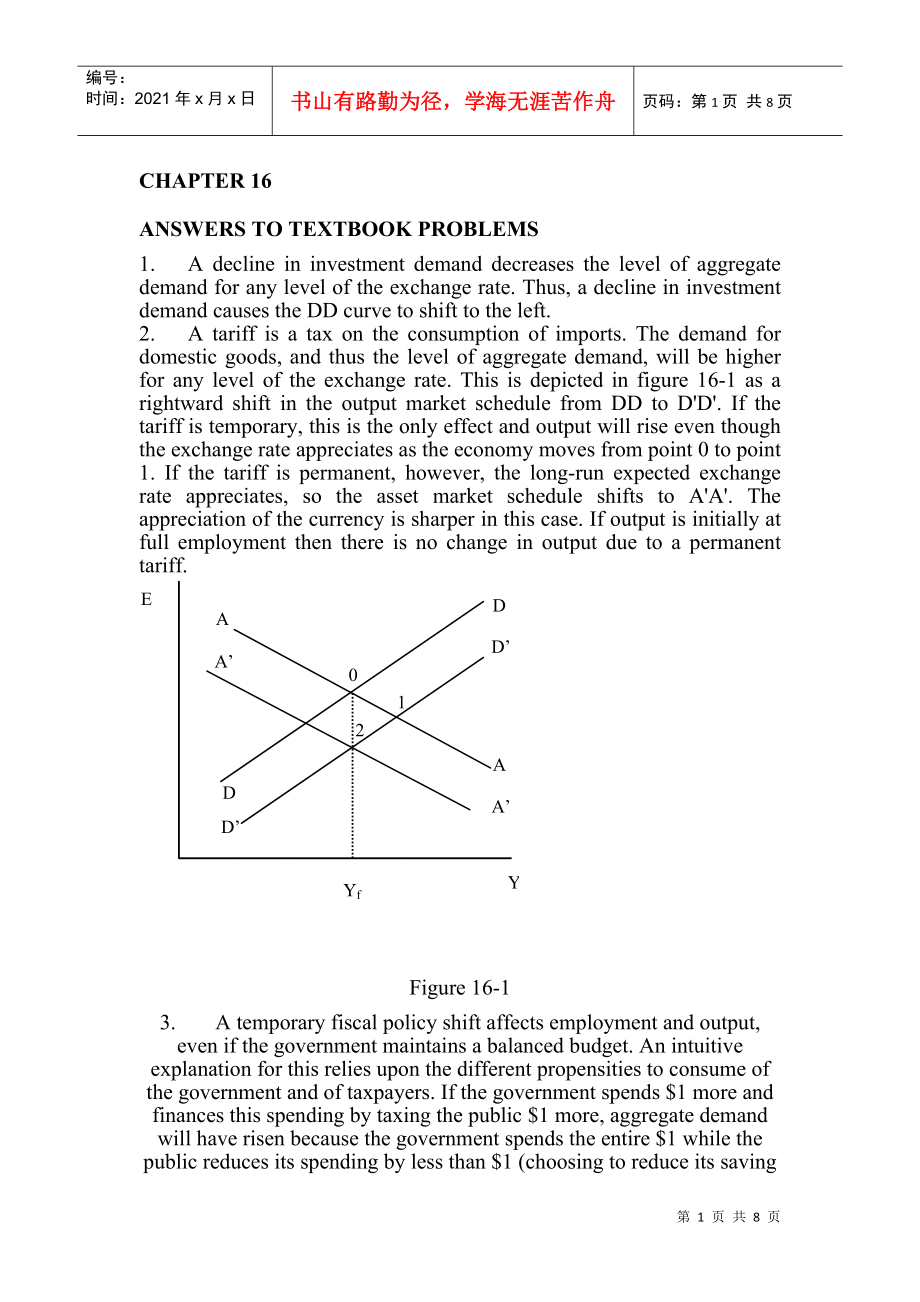
2、umption of imports. The demand for domestic goods, and thus the level of aggregate demand, will be higher for any level of the exchange rate. This is depicted in figure 16-1 as a rightward shift in the output market schedule from DD to DD. If the tariff is temporary, this is the only effect and outp

3、ut will rise even though the exchange rate appreciates as the economy moves from point 0 to point 1. If the tariff is permanent, however, the long-run expected exchange rate appreciates, so the asset market schedule shifts to AA. The appreciation of the currency is sharper in this case. If output is

4、 initially at full employment then there is no change in output due to a permanent tariff.Figure 16-13. A temporary fiscal policy shift affects employment and output, even if the government maintains a balanced budget. An intuitive explanation for this relies upon the different propensities to consu

5、me of the government and of taxpayers. If the government spends $1 more and finances this spending by taxing the public $1 more, aggregate demand will have risen because the government spends the entire $1 while the public reduces its spending by less than $1 (choosing to reduce its saving as well a

6、s its consumption). The ultimate effect on aggregate demand is even larger than this first round difference between government and public spending propensities, since the first round generates subsequent spending (Of course, currency appreciation still prevents permanent fiscal shifts from affecting

7、 output in our model.) 4. A permanent fall in private aggregate demand causes the DD curve to shift inward and to the left and, because the expected future exchange rate depreciates, the AA curve shifts outward and to the right. These two shifts result in no effect on output, however, for the same r

8、eason that a permanent fiscal expansion has no effect on output. The net effect is a depreciation in the nominal exchange rate and, because prices will not change, a corresponding real exchange rate depreciation. A macroeconomic policy response to this event would not be warranted. Figure 16-25. Fig

9、ure 16-2 can be used to show that any permanent fiscal expansion worsens the current account. In this diagram, the schedule XX represents combinations of the exchange rate and income for which the current account is in balance. Points above and to the left of XX represent current account surplus and

10、 points below and to the right represent current account deficit. A permanent fiscal expansion shifts the DD curve to DD and, because of the effect on the long run exchange rate, the AA curve shifts to AA. The equilibrium point moves from 0, where the current account is in balance, to 1, where there

11、 is a current account deficit. If, instead, there was a temporary fiscal expansion of the same size, the AA curve would not shift and the new equilibrium would be at point 2 where there is a current account deficit, although it is smaller than the current account deficit at point 1. 6. A temporary t

12、ax cut shifts the DD curve to the right and, in the absence of monetization, has no effect on the AA curve. In figure 16-3, this is depicted as a shift in the DD curve to DD, with the equilibrium moving from point 0 to point 1. If the deficit is financed by future monetization, the resulting expecte

13、d long-run nominal depreciation of the currency causes the AA curve to shift to the right to AA which gives us the equilibrium point 2. The net effect on the exchange rate is ambiguous, but output certainly increases more than in the case of a pure fiscal shift.Figure 16-37. A currency depreciation

14、accompanied by a deterioration in the current account balance could be caused by factors other than a J-curve. For example, a fall in foreign demand for domestic products worsens the current account and also lowers aggregate demand, depreciating the currency. In terms of figure 16-4, DD and XX under

15、go equal vertical shifts, to DD and XX, respectively, resulting in a current account deficit as the equilibrium moves from point 0 to point 1. To detect a J-curve, one might check whether the prices of imports in terms of domestic goods rise when the currency is depreciating, offsetting a decline in

16、 import volume and a rise in export volume. Figure 16-48. The expansionary money supply announcement causes a depreciation in the expected long-run exchange rate and shifts the AA curve to the right. This leads to an immediate increase in output and a currency depreciation. The effects of the antici

17、pated policy action thus precede the policys actual implementation. Figure 16-59. If exchange rate pass-through is incomplete in the short-run then the DD curve becomes steeper; a given appreciation of the exchange rate crowds out less imports because the foreign currency price of these imports fall

18、s concurrent with the appreciation of the currency. In this case, a permanent fiscal expansion both shifts out the DD curve and, because of pricing behavior by foreign exporters, makes it steeper. This results in an increase in output along with a current account deficit, as depicted in figure 16-5

19、by a shift from DD to DD which shifts the equilibrium point from 0 to 1. Over time, as the foreign currency price of imports rise, the slope of the DD returns to its original value, which reduces output and offsets, to some extent, the current account deficit. In the diagram, this is depicted as a m

20、ovement from point 1 to point 2 with a flattening of the output market curve from DD to DD. Thus, low government and private savings caused the current account deficit, but incomplete pass-through exacerbated the initial effect on the current account.10. The DD curve might be negatively sloped in th

21、e very short run if there is a J-curve, though the absolute value of its slope would probably exceed that of AA. This is depicted in figure 16-6. The effects of a temporary fiscal expansion, depicted as a shift in the output market curve to DD, would not be altered since it would still expand output

22、 and appreciate the currency in this case (the equilibrium point moves from 0 to 1). Figure 16-6Monetary expansion, however, while depreciating the currency, would reduce output in the very short run. This is shown by a shift in the AA curve to AA and a movement in the equilibrium point from 0 to 2.

23、 Only after some time would the expansionary effect of monetary policy take hold (assuming the domestic price level did not react too quickly). 11. The derivation of the Marshall-Lerner condition uses the assumption of a balanced current account to substitute EX for (q x EX*). We cannot make this su

24、bstitution when the current account is not initially zero. Instead, we define the variable z = (q x EX*)/EX. This variable is the ratio of imports to exports, denominated in common units. When there is a current account surplus, z will be less than 1 and when there is a current account deficit z wil

25、l exceed 1. It is possible to take total derivatives of each side of the equation CA = EX - q EX* and derive a general Marshall-Lerner condition as n + z n* z, where n and n* are as defined in the appendix. The balanced current account (z=1) Marshall-Lerner condition is a special case of this genera

26、l condition. A depreciation is less likely to improve the current account the larger its initial deficit when n* is less than 1. Conversely, a depreciation is more likely to cause an improvement in the current account the larger its initial surplus, again for values of n* less than 1. Figure 16-712.

27、 If imports constitute part of the CPI then a fall in import prices due to an appreciation of the currency will cause the overall price level to decline. The fall in the price level raises real balances. As shown in diagram 16-7, the shift in the output market curve from DD to DD is matched by an in

28、ward shift of the asset market equilibrium curve. If import prices are not in the CPI and the currency appreciation does not affect the price level, the asset market curve shifts to AA and there is no effect on output, even in the short run. If, however, the overall price level falls due to the appr

29、eciation, the shift in the asset market curve is smaller, to AA, and the initial equilibrium point, point 1, has higher output than the original equilibrium at point 0. Over time, prices rise when output exceeds its long-run level, causing a shift in the asset market equilibrium curve from AA to AA,

30、 which returns output to its long-run level. 13. An increase in the risk premium shifts the asset market curve out and to the right, all else equal. A permanent increase in government spending shifts the asset market curve in and to the right since it causes the expected future exchange rate to appr

31、eciate. A permanent rise in government spending also causes the goods market curve to shift down and to the right since it raises aggregate demand. In the case where there is no risk premium, the new intersection of the DD and AA curve after a permanent increase in government spending is at the full

32、-employment level of output since this is the only level consistent with no change in the long-run price level. In the case discussed in this question, however, the nominal interest rate rises with the increase in the risk premium. Therefore, output must also be higher than the original level of ful

33、l-employment output; as compared to the case in the text, the AA curve does not shift by as much so output rises.14. Suppose output is initially at full employment. A permanent change in fiscal policy will cause both the AA and DD curves to shift such that there is no effect on output. Now consider

34、the case where the economy is not initially at full employment. A permanent change in fiscal policy shifts the AA curve because of its effect on the long-run exchange rate and shifts the DD curve because of its effect on expenditures. There is no reason, however, for output to remain constant in thi

35、s case since its initial value is not equal to its long-run level, and thus an argument like the one in the text that shows the neutrality of permanent fiscal policy on output does not carry through. In fact, we might expect that an economy that begins in a recession (below Yf) would be stimulated b

36、ack towards Yf by a positive permanent fiscal shock. If Y does rise permanently, we would expect a permanent drop in the price level (since M is constant). This fall in P in the long run would move AA and DD both out. We could also consider the fact that in the case where we begin at full employment

37、 and there is no impact on Y, AA was shifting back due to the real appreciation necessitated by the increase in demand for home products (as a result of the increase in G). If there is a permanent increase in Y, there has also been a relative supply increase which can offset the relative demand incr

38、ease and weaken the need for a real appreciation. Because of this, AA would shift back by less. We do not know the exact effect without knowing how far the lines originally move (the size of the shock), but we do know that without the restriction that Y is unchanged in the long run, the argument in

39、the text collapses and we can have both short run and long run effects on Y.15. The text shows output cannot rise following a permanent fiscal expansion if output is initially at its long-run level. Using a similar argument, we can show that output cannot fall from its initial long-run level followi

40、ng a permanent fiscal expansion. A permanent fiscal expansion cannot have an effect on the long-run price level since there is no effect on the money supply or the long-run values of the domestic interest rate and output. When output is initially at its long-run level, R equals R*, Y equals Yf and r

41、eal balances are unchanged in the short run. If output did fall, there would be excess money supply and the domestic interest rate would have to fall, but this would imply an expected appreciation of the currency since the interest differential (R - R*) would then be negative. This, however, could o

42、nly occur if the currency appreciates in real terms as output rises and the economy returns to long-run equilibrium. This appreciation, however, would cause further unemployment and output would not rise and return back to Yf. As with the example in the text, this contradiction is only resolved if output remains at Yf. 第 8 页 共 8 页